Mathématiques pour les IFS, fractales & jeu du chaos
Cadre mathématique et démonstrations
Distances
Une distance est une application
-
 (symétrie)
-
 (séparation)
- Pour tous
 ,
,  et
et  ,
,
 (inégalité triangulaire)
Par exemple, en géométrie dans le plan
-

-

- pour tout point
 ,
, 
Si le plan est rapporté à un repère orthonormé, et que
est une distance, la distance euclidienne.
On peut définir de nombreuses distances, suivant le contexte, les éléments dont on cherche à mesurer la distance: distances entre des points, entre des fonctions, entre des matrices, … et aussi, ce qui nous intéresse plus ici, entre des ensembles géométriques de points (c'est-à-dire des figures géométriques, ou encore des images).
Distance et norme
Un espace normé est un espace muni d'une norme, un espace métrique est lui muni d'une distance.Une norme, notée en général
La réciproque n'est par contre pas toujours vraie: une distance peut ne pas découler d'une norme.
En d'autres termes, un espace normé est nécessairement aussi métrisé (ou métrique), par contre un espace métrique n'est pas toujours normé.
La notion de norme est plus fine que celle de distance.
Une distance entre éléments d'un espace permet par contre aussi d'induire un distance entre des ensembles d'éléments: c'est la distance de Hausdorff.
Distance de Hausdorff
Définition et propriété
En traitement d'image par exemple, on cherche à donner un sens à la proximité de deux images entre elles: deux images, par exemple une floue et la même filtrée et plus nette, sont elles "proches" entre elles.
Plus précisément sur une série d'images filtrées et traîtées, laquelle est la plus "proche" de l'image souhaitée.
Comment quantifier cette "proximité" ? Comment vérifier que deux motifs, ou parties d'images sont identiques ?
Une distance est un outil mathématique qui permet exactement de définir la notion de proximité.
La distance de Hausdorff est une distance qui permet de mesurer la différence entre des ensembles, de points par exemple (c'est à dire des images).
Pour définir cette distance de Hausdorff, on a besoin de la définition de la distance d'un point à un ensemble, puis de celle de voisinage d'un ensemble.
Définition: distance d'un point à un ensemble
La distance d'un point  à un ensemble
  est la plus petite des
distances entre
est la plus petite des
distances entre  et les points de
  :
:
![\[d(x,A)=\inf\Bigl\{ d(x,y) , y\in A \Bigr\}\]](fich-chaos-IMG/200.png)
(3,1)
\rput(1.1,2){\Large$A$}
\rput(0,5){\large$\tm$}\rput(-.25,5.2){\large$x$}
\psline[linewidth=1.5pt,linecolor=magenta,arrowsize=8.5pt]{<->}(0,5)(0.4,2.82)
\rput(1.1,4){\large\magenta$d(x,A)$}
\end{pspicture}\]](fich-chaos-IMG/201.png)
Définition: Voisinage
On appelle voisinage, ou  d'un ensemble
  de points du plan
l'ensemble des points
de points du plan
l'ensemble des points
![\[V_r(A)=\Bigl\{ x \text{ tel que } d(x,A)<r \Bigr\}\]](fich-chaos-IMG/204.png)
(3,1)
\rput(1.1,2){\Large$A$}
\psellipse[fillstyle=vlines,hatchsep=2.1em,hatchcolor=blue](2,2)(4,1.9)
\psellipse[linestyle=none,fillstyle=solid,fillcolor=white](.42,3.15)(.29,.28)
\psellipse[linestyle=none,fillstyle=solid,fillcolor=white](.42,3.15)(.29,.28)
\psellipse[linestyle=none,fillstyle=solid,fillcolor=white](4,3.15)(.5,.28)
\psline[linewidth=2pt,linecolor=magenta,arrowsize=7pt]{<->}(4,2.7)(4.5,3.5)
\rput(4,3.2){\large\magenta$r$}
\psellipse[linestyle=none,fillstyle=solid,fillcolor=white](.42,3.15)(.29,.28)
\rput(.2,3.1){\large\blue$V_r(A)$}
\end{pspicture}\]](fich-chaos-IMG/205.png)
Définition: distance de Hausdorff
La distance de Hausdorff entre deux ensembles  et
et  est
définie par
est
définie par
![\[d_H(A,B)=\inf\Bigl\{ r>0 \text{ tel que }
A\subset V_r(B) \text{ et } B\subset V_r(A) \Bigr\}
\]](fich-chaos-IMG/208.png)
La distance de Hausdorff est définie à partir de la notion de voisinage, qui elle-même est dépend de la distance dans l'espace considéré.
La distance de Hausdorff n'est pas une distance sur tous les ensembles; par exemple, pour des ensembles de points non-bornés, la distance de Hausdorff n'est pas définie (ou vaut dans ce cas l'infini).
Par contre, en se limitant aux ensembles compacts, qui sont dans le plan les ensembles fermés et bornés, la distance de Hausdorff définie bien une distance: en notant
Propriété: La distance de Hausdorff est une distance
sur  .
.
Démonstration.
Il faut démontrer les trois propriétés d'une distance.
- Symétrie: elle est évidente, la définition de la distance étant
elle même symétrique:
 .
.
- Séparation: Supposons
 et
et  sont deux ensembles
compacts tels que
sont deux ensembles
compacts tels que  .
.
Cela signifie que pour tout , on a
 (et de même
  ).
).
Prenons par exemple , tel que
 .
.
Alors, il existe tel que
  .
.
Comme pour tous entiers et
et  on a d'après l'inégalité triangulaire
 ,
la suite
,
la suite  est de Cauchy.
Comme on est dans un espace complet, cette suite converge,
ce qui signifie qu'il existe
est de Cauchy.
Comme on est dans un espace complet, cette suite converge,
ce qui signifie qu'il existe  tel que
 .
.
Enfin, comme est compact, et que pour tout
  ,
,
 , on a aussi que
  .
.
Ainsi, en passant à la limite, on obtient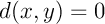 soit donc
 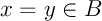 .
.
Finalement, on a donc .
.
En raisonnant de même en interchangeant et
et  ,
on obtient aussi
,
on obtient aussi  , et donc
 .
.
- Inégalité triangulaire:
soit
 ,
,  et
et  trois ensembles compacts,
on cherche à montrer que,
trois ensembles compacts,
on cherche à montrer que,
 .
.
On note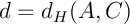 ,
,  et
et  .
.
On a alors et
et  .
.
Ainsi,
Or d'après le lemme suivant.
Ainsi, .
.
De même, on arrive symétriquement à .
.
On a ainsi, .
.
Lemme:
Pour tout ensemble  , et
, et  et
et  ,
on a
,
on a
 .
.
Démonstration.
Soit  ,
alors il existe
,
alors il existe  tel que
 .
.
De même, comme , il existe
  tel que
  .
.
D'après l'inégalité triangulaire, on a ,
ce qui signifie que
,
ce qui signifie que
 .
.
De même, comme
D'après l'inégalité triangulaire, on a
Exemples
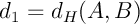
Exemple 1:
On cherche par exemple la distance de Hausdorff entre les ensembles
(2,2)(-2,2)(-2,-2)
\pscircle[linecolor=red,fillstyle=hlines,hatchcolor=red,hatchsep=1.1em](1,.5){2}
\pscircle[fillstyle=solid,fillcolor=white,linestyle=none](-1.7,-1.6){.25}
\rput(-1.7,-1.5){\large\blue$A$}
\rput(2.5,.3){\large\red$B$}
\end{pspicture}\]](fich-chaos-IMG/270.png)
On trace le plus petit voisinage de
(2,2)(-2,2)(-2,-2)
\pscircle[fillstyle=solid,fillcolor=white,linestyle=none](-1.7,-1.6){.25}
\rput(-1.7,-1.5){\large\blue$A$}
\pscircle[linecolor=red,fillstyle=hlines,hatchcolor=red,hatchsep=1.1em](1,.5){2}
\pscircle[fillstyle=solid,fillcolor=white,,linestyle=none](2.5,.3){.3}
\rput(2.5,.3){\large\red$B$}
\psline[arrowsize=6pt,linecolor=blue,linewidth=1.5pt]{<->}(-3,1)(-2,1)
\rput(-2.5,1.3){\large\blue$r_1$}
\psline(3,-2)(3,2)
\psline(2,3)(-2,3)
\psline(-3,2)(-3,-2)
\psline(-2,-3)(2,-3)
\psarc(2,2){1}{0}{90}
\psarc(-2,2){1}{90}{180}
\psarc(-2,-2){1}{180}{270}
\psarc(2,-2){1}{270}{360}
\end{pspicture}\]](fich-chaos-IMG/275.png)
(12,2)(8,2)(8,-2)
\pscircle[linecolor=red,fillstyle=hlines,hatchcolor=red,hatchsep=1.1em](11,.5){2}
\psline[arrowsize=6pt,linecolor=red,linewidth=1.5pt]{<->}(13,.5)(14.95,.5)
\rput(14,.8){\large\red$r_2$}
\pscircle(11,.5){3.95}
\pscircle[fillstyle=solid,fillcolor=white,linestyle=none](8.3,-1.6){.25}
\rput(8.3,-1.5){\large\blue$A$}
\pscircle[fillstyle=solid,fillcolor=white,,linestyle=none](12.5,.3){.3}
\rput(12.5,.3){\large\red$B$}
\end{pspicture}\]](fich-chaos-IMG/276.png)
On a ici
Par contre
Ainsi,
Exemple 2: La distance de Hausdorff est une distance sur
Par exemple, si
Application contractante
Une application contractante est une application qui rapproche les points, c'est-à-dire que les images de deux points sont plus proches que les points eux-même. Plus précisément,
Définition: application contractante
Une application  est contractante
si il existe un nombre réel
est contractante
si il existe un nombre réel  tel que, pour tous
  et
et  ,
,
![\[d\left( f(x),f(y)\rp\leqslant k\,d\left( x,y\rp\]](fich-chaos-IMG/296.png)
Il faut ici faire attention à la distance utilisée. Ce n'est pas forcément la même distance à gauche et à droite de l'inégalité précédente. La distance euclidienne peut être utilisée s'il s'agit de distance entre points du plan, celle de Hausdorff pour des ensembles de points.
L'opérateur de Hutchinson  est contractant
On peut maintenant revenir sur l'opérateur de Hutchinson.
Propriété: L'opérateur de Hutchinson  est contractant
sur
est contractant
sur  pour la distance de Hausdorff.
Pour démontrer cette propriété, qui est la propriété fondamentale garantissant l'existence et l'unicité de l'attracteur d'un IFS, on a besoin de résultats intermédiaires.
Lemme 1:
Pour tous ensemble  et
et  , et réel
  ,
on a
,
on a  .
.
Démonstration.
Soit  .
.
 et
et  jouant des rôles symétriques, on peut supposer
 .
.
Il existe donc tel que
  .
.
Mais alors, on a aussi et toujours
  ,
ce qui signifie que
,
ce qui signifie que  .
.
Il existe donc
Mais alors, on a aussi
Lemme 2:
Soit  une contraction du plan de rapport
  ,
alors, pour tous ensembles
,
alors, pour tous ensembles  et
et  ,
,
![\[d_H\left( f(A),f(B)\rp\leqslant d_H(A,B)\]](fich-chaos-IMG/317.png)
Démonstration.
On pose  .
.
Soit , alors il existe
  tel que
  .
.
Comme , on a
  ,
et donc il existe
,
et donc il existe  tel que
 .
On pose alors
.
On pose alors  et on a, comme
  est
est
 -contractante,
![\[
d\left( a',b'\rp=d\left( f(a),f(b)\rp
\leqslant r d(a,b)
\leqslant rk\]](fich-chaos-IMG/329.png)
En d'autres termes, on a trouvé que pour tout ,
il existe
,
il existe  tel que
 ,
d'où
,
d'où  .
.
De même, en inversant les rôles de et
et  ,
on aboutit à
,
on aboutit à  .
.
On a donc finalement, .
.
Soit
Comme
En d'autres termes, on a trouvé que pour tout
De même, en inversant les rôles de
On a donc finalement,
Lemme 3:
Pour tous compacts  et
et  du plan,
![\[d_H\left( A\cup B,C\cup D\rp\leqslant \max\Bigl\{d_H(A,C),d_H(B,D)\Bigr\}\]](fich-chaos-IMG/340.png)
Démonstration.
On pose  et
et  .
.
On a alors, par définition de la distance de Hausdorff,
![\[A\subset V_d(C) \ \text{ et } \ C\subset V_d(A)\]](fich-chaos-IMG/343.png)
et de même
![\[B\subset V_{d'}(D) \ \text{ et } \ D\subset V_{d'}(B)\]](fich-chaos-IMG/344.png)
et donc, en notant ,
,
![\[A\subset V_k(C) \ \text{ et } \ C\subset V_k(A)\]](fich-chaos-IMG/346.png)
et de même
![\[B\subset V_k(D) \ \text{ et } \ D\subset V_k(B)\]](fich-chaos-IMG/347.png)
Or, d'après le lemme 1,
et donc,
![\[A\cup B\subset V_k(C)\cup V_k(D) \subset V_k\left( C\cup D\rp\]](fich-chaos-IMG/349.png)
et de même
![\[C\cup D\subset V_k(A)\cup V_k(B) \subset V_k\left( A\cup B\rp\]](fich-chaos-IMG/350.png)
et on a donc,
![\[d_H\left( A\cup B,C\cup D\rp\leqslant k=\max\left\{}\newcommand{\ra}{\right\} d,d'\ra
=\max\Bigl\{d_H(A,C),d_H(B,D)\Bigr\}\]](fich-chaos-IMG/351.png)
On a alors, par définition de la distance de Hausdorff,
et de même
et donc, en notant
et de même
Or, d'après le lemme 1,
et donc,
et de même
et on a donc,
On peut maintenant démontrer la propriété fondamentale sur l'opérateur de Hutchinson.
Démonstration.
Soit  et
et  deux ensembles compacts du plan, alors
![\[d_H\left( F(A),F(B)\right)
=d_H\Bigl( f_1(A)\cup f_2(A)\cup\dots\cup f_N(A),
f_1(B)\cup f_2(B)\cup\dots\cup f_N(B)\Bigr)
\]](fich-chaos-IMG/354.png)
soit, en utilisant le lemme 3,
![\[\begin{array}{ll}
d_H\left( F(A),F(B)\right)
&=d_H\Bigl( f_1(A)\cup D,
f_1(B)\cup E\Bigr)\\[1em]
&\leqslant\max\Bigl\{ d_H\Bigl( f_1(A),f_1(B)\Bigr) ,
d_H\left( D,E\right) \Bigr\}
\enar\]](fich-chaos-IMG/355.png)
avec et
et  .
.
Or, comme est
est  -contractante, d'après le lemme 2,
 ,
d'où
,
d'où
![\[d_H\left( F(A),F(B)\right)
\leqslant \max\Bigl\{ r_1d_H (A,B), d_H(D,E)\Bigr\}\]](fich-chaos-IMG/361.png)
On continue avec les ensemble et
et  :
:
![\[\begin{array}{ll}
d_H(D,E)
&=d_H\Bigl( f_2(A)\cup f_3(A)\cup\dots\cup f_N(A),
f_2(B)\cup f_3(B)\cup\dots\cup f_N(B)\Bigr) \\[1em]
&=d_H\Bigl( f_2(A)\cup D',f_2(B)\cup E'\Bigr)
\enar\]](fich-chaos-IMG/364.png)
avec et
et  d'où, à nouveau à l'aide du lemme 3,
![\[\begin{array}{ll}
d_H(D,E)\leqslant
\max\Bigl\{ d_H\Bigl(f_2(A),f_2(B)\Bigr),d_H\left( D',E'\rp\Bigr\}
\enar\]](fich-chaos-IMG/367.png)
avec, d'après le lemme 2, .
.
En poursuivant ainsi, on arrive donc enfin à:
![\[\begin{array}{ll}
d_H\left( F(A),F(B)\rp&\leqslant
\max\Bigl\{ r_1d_H(A,B),r_2d_H(A,B),\dots,r_Nd_H(A,B)\Bigr\}\\[1.2em]
&=\max\Bigl\{ r_1,r_2,\dots,r_N\Bigr\} d_H(A,B)\\[1em]
&=rd_H(A,B)
\enar\]](fich-chaos-IMG/369.png)
avec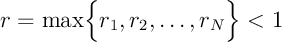 .
.
soit, en utilisant le lemme 3,
avec
Or, comme
On continue avec les ensemble
avec
avec, d'après le lemme 2,
En poursuivant ainsi, on arrive donc enfin à:
avec
Théorème du point fixe
Il existe de nombreux théorèmes du point fixe en analyse. Ils permettent de démontrer l'existence et l'unicité d'une solution à des problèmes, en fournissant de plus une méthode constructive pour les déterminer (ou du moins en donner une approximation, avec une précsion souhaitée).
Le théorème du point fixe utilisé ici est celui de Banach, ou de Picard, et se place dans un espace métrique complet.
Un espace métrique est un espace dans lequel on peut mesurer, c'est-à-dire muni d'une distance telle que vue précédemment. On note justement
Théorème du point fixe de Banach / Picard:
Une application  contractante dans un espace métrique complet
admet un unique point fixe, c'est-à-dire un unique
contractante dans un espace métrique complet
admet un unique point fixe, c'est-à-dire un unique  tel que
  .
.
De plus, est la limite de toute suite
  définie
par récurrence selon
définie
par récurrence selon  .
.
On a de plus alors les majorations
![\[d\left( x_n,x\right) \leqslant k^n d\left( x_0,x\right)\]](fich-chaos-IMG/378.png)
et
![\[d\left( x_n,x\right) \leqslant \dfrac{k^n}{1-k} d\left( x_0,x_1\right)\]](fich-chaos-IMG/379.png)
où est le rapport de contraction de
  .
.
De plus,
On a de plus alors les majorations
et
où
Démonstration:
Ce théorème donne deux résultats:
l'existence et l'unicité du point fixe  .
.
On démontre les deux séparemment.
On démontre les deux séparemment.
- Unicité. Supposons au contraire qu'il y ait deux points fixes
 et
et  :
:  et
et  avec
avec  .
.
On aurait alors or, comme
  est contractance de rapport
  ,
on a aussi
,
on a aussi  .
.
On devrait donc avoir ce qui est impossible.
Ainsi, si un point fixe existe, il est nécessairement unique.
- Existence.
L'existence se démontre par le procédé construcif même utilisé tout au long de ces pages: soit une suite définie par récurrence par
  .
.
Alors on, our tout entier et
et 
![\[d\left( x_n,x_p\rp\leqslant \dfrac{k^n}{1-k}d(x_0,x_1)\]](fich-chaos-IMG/397.png)
avec, comme ,
,
 .
.
Ceci montre que la suite est une suite de Cauchy,
et alors, comme on est dans un espace complet,
la suite converge donc vers une limite
est une suite de Cauchy,
et alors, comme on est dans un espace complet,
la suite converge donc vers une limite  .
.
Par unicité du point fixe, on voit donc que ce procédé constructif ne dépend pas du point initial de la suite:
pour tout
de la suite:
pour tout  la suite
  ainsi définie converge,
vers le point fixe de
ainsi définie converge,
vers le point fixe de  .
.