Construction de la fonction exponentielle -- Méthode d'Euler

Y. Morel

La fonction exponentielle est l'unique fonction dérivable sur $\R$ qui vérifie

. (cf. cours)

À partir de ces deux seules informations, on peut construire approximativement la fonction et sa courbe, c'est-à-dire qu'on peut calculer approximativement la valeur

pour tout nombre réel

Méthode d'Euler: approximation des valeurs de

L'information principale sur

concerne sa dérivée

. Or la dérivée de

est la limite du taux de variation:

$f'(x)=\lim_{h\to0}\dfrac{f(x+h)-f(x)}h$

Ainsi, pour un nombre

"assez petit" on peut écrire l'approximation

$f'(x)\simeq\dfrac{f(x+h)-f(x)}h$

Plus

est petit, meilleure est cette approximation.

Maintenant, comme

, on a donc

$f(x)\simeq\dfrac{f(x+h)-f(x)}h$

soit, en isolant

$f(x+h)\simeq hf(x)+f(x)$

ou encore

$f(x+h)\simeq(1+h)f(x)$

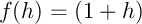
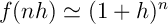
En particulier, en partant de

, on obtient

$f(h)=(1+h)f(0)$

et comme

$f(h)=(1+h)$

On a donc

pour ,
pour , $f(h+h)=f(2h)\simeq(1+h)f(h)=(1+h)^2$ ,
pour , $f(2h+h)=f(3h)\simeq(1+h)f(2h)=(1+h)^3$ ,
… …
pour tout entier , $f(nh)\simeq(1+h)^n$

On balaye ainsi, par pas de

, les valeurs prises par la fonction

.

Pour calculer une valeur particulière

, il suffit d'adapter ce pas: si

est un nombre réel quelconque, et

un entier naturel, il suffit de poser $h=\dfrac{x}n$ pour avoir

, et alors, avec le résultat précédent,

$f(x)=f(nh)\simeq(1+h)^n$

soit finalement

$f(x)\simeq\lp1+\dfrac{x}n\rp^n$

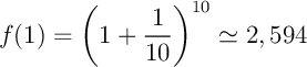
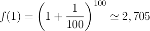
Calcule de $\exp(1)$

On peut maintenant donner une valeur approchée de

. On arrondissant les valeurs à $10^{-3}$ près, on obtient:

Pour , $f(1)=\lp1+\dfrac1{10}\rp^{10}\simeq 2,594$
Pour , $f(1)=\lp1+\dfrac1{100}\rp^{100}\simeq 2,705$
Pour , $f(1)=\lp1+\dfrac1{1000}\rp^{1000}\simeq 2,717$
…

Valeurs qu'on compare bien sûr à la valeur de $\exp(1)$ , connue par toute calculatrice ou ordinateur^*:

$\exp(1)\simeq 2,718$

Courbe représentative de l'exponentielle

On peut de même calculer toute valeur souhaitée

de la même façon, et tracer ainsi l'allure de la courbe représentative de la fonction exponentielle, obtenue comme courbe limite de la courbe de la fonction

lorsque $n\to+\infty$ .

On trace donc la courbe de la "vraie"^** fonction exponentielle et celles des fonctions définies par $f(x)=\lp1+\dfrac{x}n\rp^n$ pour différentes valeurs de l'entier

$\psset{xunit=1cm,yunit=.15cm,arrowsize=8pt}\begin{pspicture*}(-1.5,-5)(4,60) \psline{->}(-1.4,0)(3.9,0) \psline{->}(0,-.5)(0,56) \multido{\i=-1+1}{5}{\psline(\i,-1)(\i,1)\rput(\i,-2.4){$\i$}} \multido{\i=10+10}{5}{\psline(-.1,\i)(.1,\i)\rput[r](-.2,\i){$\i$}} \psplot[linewidth=1.8pt,linecolor=red]{-1}{8}{2.71828 x exp} \psplot[linewidth=1.8pt,linecolor=blue]{-1}{6}{1 x 10 div add 10 exp} \psplot[linewidth=1.8pt,linecolor=cyan]{-1}{6}{1 x 50 div add 50 exp} \psplot[linewidth=1.8pt,linecolor=magenta]{-1}{7.6}{1 x 5 div add 5 exp} %\pspolgon( \psline[linewidth=2.5pt,linecolor=red](.5,45)(1,45)\rput[l](1.2,44){$\exp$} \psline[linewidth=2.5pt,linecolor=cyan](.5,41)(1,41)\rput[l](1.2,41){$n=50$} \psline[linewidth=2.5pt,linecolor=blue](.5,37)(1,37)\rput[l](1.2,37){$n=10$} \psline[linewidth=2.5pt,linecolor=magenta](.5,33)(1,33)\rput[l](1.2,33){$n=5$} \end{pspicture*}$

*: Pour utiliser la fonction exponentielle en python (et d'autres comme le logarithme, les fonctions trigonométriques, … ), il faut la charger depuis la bibliothèque des fonctions mathéamtiques: from math import exp
exp(1)
**: La fonction exponentielle n'a pas d'expression algébrique "simple" (comme la fonction carré, un polynôme …).
La "vraie courbe" de l'exponentielle est en fait tracée en utilisant des calculs approchés, comme ceux menés ici.
Les méthodes de calcul des valeurs de l'exponentielle par une calculatrice ou un ordinateur sont juste plus efficaces: c'est-à-dire la précision meilleure qu'avec la méthode d'Euler et pour un nombre plus faible de calculs.
Trouver ce genre de méthodes plus efficaces est le champ mathématique qui s'appelle l'analyse numérique.

Voir aussi: